We will build a simple form of Object Recognition System. Although the example we’ll use is very simple, it reflects many of the same key machine learning concepts that go into building real-world commercial systems.
About the Dataset
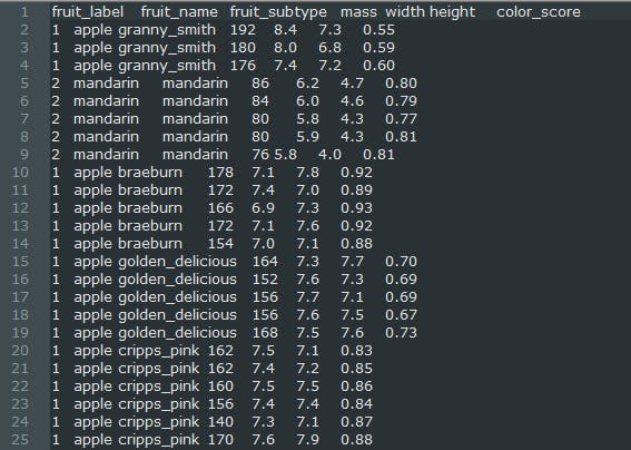
The dataset we will use is a small, very simple, for training a classifier to distinguish between distinct types of fruit.
To create the original dataset, we go to a nearby store, bought a few dozen oranges, lemons, and apples of different varieties, and recorded their measurements in a table. We notice the height and the width, estimated their mass.
We’ve formatted data slightly and added one or two extra simulated features such as a color score for instructional purposes. This dataset named “fruit_data.txt”. You can find the dataset in my GitHub repository.

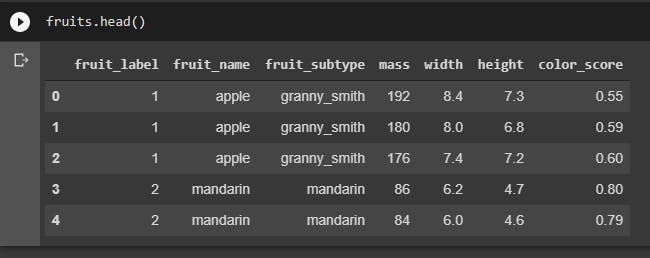
A peek of Fruits Dataset
To solve machine learning problems, you can think of the input data as a table. Each object is represented by a row, and the attributes of the object:
- Name
- Sub Type
- Measurement
- Color
The features of the fruit are represented by the values you see across the columns.
Import required Libraries
Import these modules below to proceed with the code.
%matplotlib notebook
import numpy as np
import matplotlib.pyplot as plt
import pandas as pd
from sklearn.model_selection import train_test_split
Import the Dataset
For those who are using Google Colab, use the following code snippet to import the Dataset file.
from google.colab import files
files.upload()
The first thing we will do is to load the fruit dataset file using the very handy read table command in pandas.
fruits = pd.read_table(‘fruit_data.txt’)
Now, this will read the dataset from disk, and store it into a data frame variable we’ll call fruits here.
Output:

Here we can see that each row of the dataset represents one piece of fruit as represented by several features are in the table’s columns. So, in order, the columns we see are fruit labels.
Exploratory Data Analysis
Defining a dictionary that takes a numeric fruit label as the input key. And returns a value that’s a string with the name of the fruit, and this dictionary just makes it easier to convert the output of a classifier prediction to something a person can more easily interpret, the name of a fruit in this case.
lookup_fruit_name = dict(zip(fruits.fruit_label.unique(), fruits.fruit_name.unique()))
lookup_fruit_name
Create a mapping from fruit label value to fruit name to make results easier to interpret.
To estimate how well the classifier will do on future samples, split the original dataset into two parts.
X = fruits[['height', 'width', 'mass', 'color_score']]
y = fruits['fruit_label']
We’ll have an array of labeled samples called the training set that will train the classifier.
Then we’ll hold out the remaining labeled samples and put them into a second separate array called the test set that will then evaluate the trained classifier.
X_train, X_test, y_train, y_test = train_test_split(X, y, random_state=0)
This function (random_state=0) randomly shuffles the dataset and splits off a certain percentage of the input samples for use as a training set and then puts the remaining samples into a different variable for use as a test set.
Plot Code:
from matplotlib import cm
from pandas.plotting import scatter_matrix
cmap = cm.get_cmap('gnuplot')
scatter = scatter_matrix(X_train, c= y_train, marker = 'x', s=40, hist_kwds={'bins':15}, figsize=(9,9), cmap=cmap)
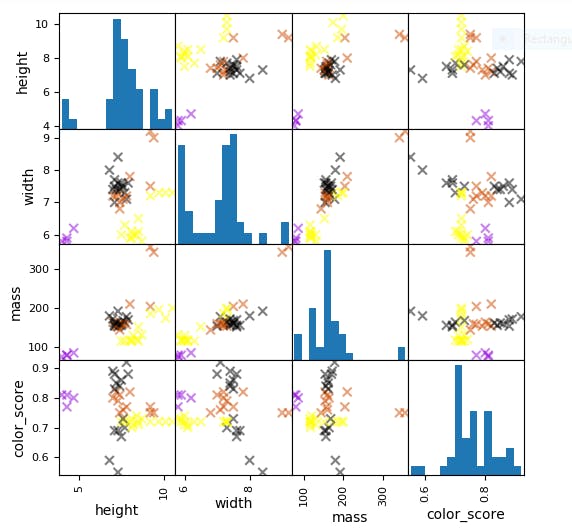
This plot shows all pairs of features and produces a scatter plot for each pair, showing how the features are correlated to each other or not.
Output:

Just by looking at this pair plot, we can already see that some pairs of features, like the height and color score in the top right corner here, are good for separating out different classes of fruit.
- Each point in the scatter plot represents a piece of fruit, colored according to the class it belongs to. And positioned using the para features assigned to that scatter plot.
- Along the diagonal is a histogram showing the distribution of feature values for that feature.
- So in this pair plot, the dimensions shown here in order are, height, width, mass. And the color score of the fruit examples in our training set.
- So the upper left corner of the histogram here shows the distribution of the height feature for all samples in the training set.
- And the scatter plot to its immediate right plots the width of each sample on the x-axis and the height of the sample on the y-axis.
Note that a pair plot like this does not show interactions between all features that might exist, just between pairs of them.
Train-Test Split
Use the mass, width, and height of the fruit as features.
X = fruits[['mass', 'width', 'height']]
y = fruits['fruit_label']
- Capital X holds the features of our data set without the label.
- Lower case y hold the corresponding labels for the instances in x.
So, this collection of features is called the feature space.
X_train, X_test, y_train, y_test = train_test_split(X, y, random_state=0)
I put the results of the train test split function into the four variables you see on the left. And these are marked as x_train, x_test, y_train, and y_test.
Classifier Object
Once we have our train-test split, we then need to create an instance of the classifier object. In this case a k-NN classifier.
from sklearn.neighbors import KNeighborsClassifier
knn = KNeighborsClassifier(n_neighbors = )
knn.fit(X_train,y_train)
We then train the classifier by passing in the training set date in X_train, and the labels in y_train to the classifiers fit method.
One simple way to assess if the classifier is likely to be good at predicting the label of future, previously unseen data instances, is to compute the classifier’s accuracy on the test set data items.
knn.score(X_test,y_test)
To do this, we use the Score Method for the classifier object. This will take the test set points as input and compute the accuracy.

It defines the accuracy as the fraction of test set the classifier correctly predicted items,.
Test Classifier
Let's test our Classifier on Unseen Data.
Example# 1
fruit_prediction = knn.predict([[20, 4.3, 5.5]])
lookup_fruit_name[fruit_prediction[0]]
Output:

Example# 2
fruit_prediction = knn.predict([[100, 6.3, 8.5]])
lookup_fruit_name[fruit_prediction[0]]
Output:

Effect of ‘k’ on Classification Accuracy
When k has a small value like 1, the classifier is good at learning the classes for individual points in the training set.
This is because when K = 1, the prediction is sensitive to
- Noise
- Outliers
- Mislabeled Data
and other variations in individual data points.
For larger values of K, the areas assigned to different classes are smoother and not as fragmented and more robust to noise in the individual points.
This is an example of what’s known as the bias-variance tradeoff.
k_range = range(1,20)
scores = []
for k in k_range:
knn = KNeighborsClassifier(n_neighbors = k)
knn.fit(X_train, y_train)
scores.append(knn.score(X_test, y_test))
plt.figure()
plt.xlabel('k')
plt.ylabel('accuracy')
plt.scatter(k_range, scores)
plt.xticks([0,5,10,15,20]);
Output

The best choice of the value of k, which is the one that leads to the highest accuracy, can vary depending on the data set.
Using a larger k suppresses the effects of noisy individual labels. But results in classification boundaries that are less detailed.
Summary
- We’ve looked at a data set, plotted some features.
2. We then took the features and learned how to compute a train test split.
3. Used that to train a classifier and
4. Used the resulting classifier to make some predictions for unfamiliar objects.
Congratulations, you’ve just created and run your first machine learning application in Python
Scope of Fruit Classification
Now you might think fruit prediction is a silly and impractical scenario. And given the limited nature of this dataset, it is a bit of a toy example. But food companies do now rely on machine learning systems that aren’t all that different in concept from the ones we’re about to build, so they can do Automated Quality Control.
For example, real systems used by fruit shipping companies that screen for rotten oranges during processing. Now the features they use in building these systems are a little more sophisticated than the ones we did in this example.
Quality control systems for rotten orange detection use ultraviolet light that can detect interior decay, which is often less visible than just by looking on the surface.
Github Repository: https://github.com/zainuleb/Applied-Machine-Learning-with-Python.github.io/tree/master/Section%201
